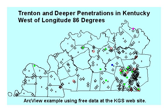
GIS example using free Kentucky data

Using ArcView to process the Oil and Gas well data file for reconnaissance investigations

Sample well location map

The instructions provided here are not intended to make you an expert in the ArcView GIS software. Visit ESRI for information on training and other resources.

Create a directory for the data and basemap files for this project, then download these files to that directory. If you have a copy of the KGSampler of Digital Data CD-ROM, these files are available in the GIS shapes\Bounds and GIS shapes\O&g directories.
1. From http://www.uky.edu/KGS/gis/geology.html, download KYOG83.ZIP
2. Other files you might want from http://www.uky.edu/KGS/gis/geology.html
  1. kyfaults24k.ZIP – surface faults digitized from the 1:24,000-scale geologic map of Kentucky
  2. CARTER1.ZIP – 1-minute Carter coordinate grid
  3. CARTER5.ZIP – 5-minute Carter coordinate grid
3. From http://www.uky.edu/KGS/gis/bounds.html, download COUNTY.ZIP
4. Other files you might want from http://www.uky.edu/KGS/gis/bounds.html
  1. QUADSKY.ZIP – grid of topographic map boundaries
Unzip the shape files to the directory you created for the download (see: http://www.winzip.com/ for WinZip)
Start ArcView with a new view (ArcView 3.2 prompts you for this when you start a new project)
Add themes to the view
1. KYOG83V2 (With the KGSampler CD-ROM, use KYOG83)
2. COUNTY
Format the View
1. In the table of contents, the oil and gas well shape file should be first (on top) with the county data following.
2. Click the check box to enable display of the county boundary file.
3. Set View | Properties | Projection category to UTM 83 and type to Zone 16. When you click OK, the Map Units should be meters and the Distance Units miles or feet. Click OK again to apply the projection.
Change the county shape file legend
1. Click the county shape file entry in the view table of contents to make it the active theme
2. Click Theme | Edit Legend
3. Double click the symbol and change the foreground color to light blue
4. Click Apply then close the Legend Editor window
Build a query and display the Trenton and deeper penetrations
1. Click the oil and gas well shape file in the view table of contents to make it the active theme
2. Click Theme | Properties
3. Click the query builder tool button (hammer with question mark icon)
4. In the list of fields, scroll down and double click on Tdfm to add it into the query window
5. On the array of operators, click the greater than or equal to button (>=)
6. Type in "365" (with the quotes). For other codes, see http://www.uky.edu/KGS/PTTC/miscdata/strtcode.htm
7. The expression should look like, parentheses included: ([Tdfm]>="365")
8. Click OK (the expression will be copied into the Definition dialog box)
9. Click OK to apply the expression
10. Click the check box for the oil and gas well shape file to display it
Select the wells west of 86 degrees longitude and make a new shape file
1. With the oil and gas well shape file the active theme, click the Query Builder button on the tool bar (hammer with question mark icon)
2. Scroll down and double click on Lonnad83 to select the field
3. Type in ".AsNumber" (without the quotes, but with the leading period)
4. Click the less than or equal to operator
5. Type in "(-86.0)" (without the quotes)
6. The expression should look like, parentheses included: ([Lonnad83].AsNumber <= (-86.0))
7. Click the New Set button and close the query window when ArcView finishes computing
8. Click Theme | Convert to Shape File
9. Enter and new theme name (like WKYPRET.SHP)
10. No, do not save the file in the projected units (leave it in decimal degrees)
11. Yes, add the new shape file to the view
12. Click on the new theme to make it active
13. Click Theme | Edit Legend
14. Click the Load button
15. Find the file KYOG83V2.AVL (KYOG83.AVL on the KGSampler CD-ROM), click OK
16. In the Load Legend window, select the Result field and make sure the All choice is checked, click OK
17. Click Apply, then close the Legend editor window
Summarize Pretrenton wells by county
1. Click the WKYPRET.SHP entry in the view’s table of contents to make it active
2. Click the open theme table button (with grid over a sheet of paper icon)
3. Click the county entry in the views table of contents to make it active
4. Click the open theme table button
5. In the Attributes of county window, click on the Shape field header (it should turn dark gray). Note the values in this field are all "Polygon."
6. In the Attributes of WKYPRET.SHP window, click on the Shape field header. The values in this field are "Point."
7. The Join button on the toolbar (to the left of the sigma icon) becomes active. Click it.
8. In the new, joined, table, scroll right and find the Name field. Click on the Name field column header.
9. Click the summarize button on the tool bar (sigma icon).
10. Change the name of the output file (if you want)
11. Click OK to create a dBase format file of the summary information. The table will be made available; see the list of tables in the project window (click Tables).
Make the summary data available and post it on the map
1. Click on the Name field in the summary data table
2. Open the table for the county theme
3. Click on the Name field in the county theme table
4. Click the Join button
5. Close all the tables
6. In the view, make the county theme active
7. Click Theme | Autolabel
8. Set the label field to count
9. Select "Use Theme’s Text Label Placement Property"
10. Click OK (Note that along the Hopkins and Muhlenberg County boundaries and in the New Madrid Bend area of Fulton County, there are several isolated polygons that get labeled with duplicate values. This can be fixed by selecting each duplicate label and pressing the delete key.)