
The Kentucky Geological Survey has archived this material, meaning (1) it is for reference, research, or recordkeeping; (2) it was created before April 24, 2026; (3) and the material has not been changed or altered since being archived. Please refer to our KGS Accessibility page for more information.
 |
 |
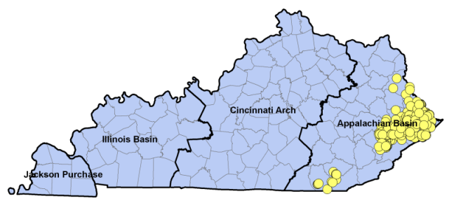
Middle and Late Devonian strata of the Appalachian Basin in the eastern United States are dominated by a sequence of black and gray shales. These low permeability, often organic-rich units are thought to be the source beds for much of the hydrocarbons produced in the basin. The shale itself can be a reservoir containing free gas in the natural fracture system, and adsorbed gas. Where the fractures in the shale are fluid filled, gas may also be dissolved in that fluid. The shale, however, is not ubiquitously productive. In areas of known production, like the Big Sandy Field of eastern Kentucky, there may exist areas of more prolific gas production. Natural gas production data sets available at the Kentucky Geological Survey will be analyzed to investigate the ability to predict the performance of Devonian shale gas wells in eastern Kentucky. In addition, these data will be spatial analyzed to identify better producing areas and make the attempt to relate those areas to geologic control affecting production.
IntroductionShales dominate the Middle and Late Devonian strata of the Appalachian Basin. Black, organic-rich, units alternate with gray shales consisting mostly of quartz and clay minerals. The shale unconformably overlies strata that varies in age from Upper Ordovician through Middle Devonian. Shale units onlap the Cincinnati Arch to the west and organic units above the Lower Huron Member of the Ohio Shale pinch out basinward. The shale ranges in thickness from 0 meters in places along the crest of the Cincinnati Arch to more than 1,097 meters (3,600 feet) in West Virginia. In the gas productive areas of Kentucky, the shale is typically 60 meters to 480 meters (200 to 1,600 feet) thick. The shale ranges in depth from the outcropping on the western margin of the basin to more than 1,200 meters (4,000 feet).
Shale gas production was discovered in eastern Kentucky circa 1892 with the drilling of wells along Beaver Creek in Floyd County. Today there are estimated to be more than 6,000 shale gas wells producing between 50 and 70 billion cubic feet of gas annually in Kentucky. Many of these wells are located in the Big Sandy gas field of Floyd, Knott, Letcher, Martin, and Pike Counties. Geologic controls and spatial distribution of better than average production are incompletely known.
The Kentucky Geological Survey has access to four data sets with direct bearing on this problem:
For data analysis, several existing resources will be used. Data compilation will be accomplished with Access and Excel (Microsoft). Graphic data analysis (histograms, graphs, etc.) will be performed in Excel with supplemental analysis and statistical testing using Python, an Open Source Software resource. Python is a scripting language that is freely available and runs on multiple computing platforms and operating systems. Scientific computing and statistical packages are available (Scipy, Numpy, and others) and have been incorporated into a single distribution, see Enthought edition of Python. Data will be spatially analyzed using the ESRI ArcGIS suite of programs (ArcMap). For cross sections, digital well log data will be processed using the GeoPlus Petra software.
A total of 304 Devonian Shale gas wells have been identified in eastern Kentucky with at least 60 months of publicly available production data and that are producing from the shale only (not commingled with the Mississippian Big Lime or other formations). Production data are availble for an additional 317 Devonian Shale gas wells in the GTI data set. The GTI data are proprietary, however, and the well identifications and locations must remain anonymous.
In eastern Kentucky, wells are commonly drilled through the Devonian Shale. The Coffee Shale (Sunbury), Brown Shale (Ohio), and White Slate (Olentangy) are consistently identified on drillers' logs of the vintage of many of the wells in the GTI production data set. The shale, of course, is penetrated when testing stratigraphically deeper pays (Silurian Big Six/Keefer, and others). Very often, wells intended to test the shallower Pennsylvanian Sands, Mississippian Maxon Sand, or the Mississippian Big Lime carbonates (Greenbriar, Monteagle, and Newman equivalents) are drilled through the shale to provide a backup should the shallower zones prove unproductive. Kentucky allows commingling of production from multiple producing zones. The result is that many wells that include a completion zone in the Devonian Shale are often completed in shallower or deeper zones and there is no way of allocating the production to a specific zone. For this project, a "shale" well is defined as a well that produces exclusively from one or more zones between the top of the Mississippian Sunbury Shale and the top of the Silurian/Devonian carbonates ("Corniferous", usually Devonian Onondaga or Silurian Salina or Lockport). This interval includes the Mississippian Sunbury Shale and Berea Sandstone, Devonian Ohio Shale (Cleveland, Three Lick Bed, Upper Huron, Middle Huron, Lower Huron, Chagrin Shales), and the Devonian Olentangy and Rhinestreet Shales (Java equivalents).
The decision to include the Berea Sand warrants clarification. Throughout much of the area where the Berea Sand is productive, it is actually a fine-grained siltstone and is considered a low permeability, "tight" sand. The Berea Sand is included as part of the shale in those wells that were stimulated (usually by explosive fracturing) in the open hole from the top of the Sunbury through the Devonian Shales. Wells completed only the Berea were excluded.
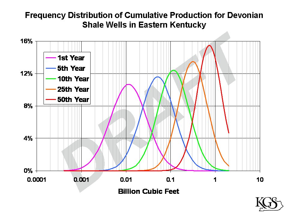
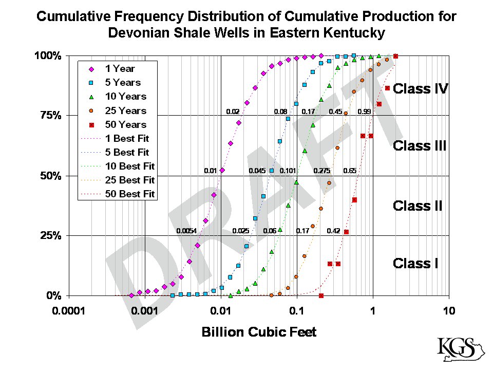
What is a "better" shale well?The performance of Devonian shale wells can only be based on volumetric criteria. Economic considerations (cost of stimulation, gathering, compression, and processing) are beyond the scope of the available data. Performance will be determined using cumulative production data derived from annual or monthly data available in the public and GTI production data sets. The first full year of production is used as the first year cumulative production. Otherwise, cumulative production is then calculated for five, 10, 25, and 50 year intervals. These data are log normally distributed as illustrated. Based on the distribution of the data, it is natural to break the data into four classes based on percentiles of the cumulative distribution.
| Class | Percentile boundaries |
|---|---|
| I | <25th |
| II | >=25th to <50th |
| III | >=50th to <75th |
| IV | >=75th |
| Cumulative Years | 25th %tile (Bcf) | 50th %tile (Bcf) | 75th %tile (Bcf) |
|---|---|---|---|
| 1 | 0.0054 | 0.01 | 0.02 |
| 5 | 0.025 | 0.045 | 0.08 |
| 10 | 0.06 | 0.101 | 0.17 |
| 25 | 0.17 | 0.275 | 0.45 |
| 50 | 0.42 | 0.65 | 0.99 |
 |
 |
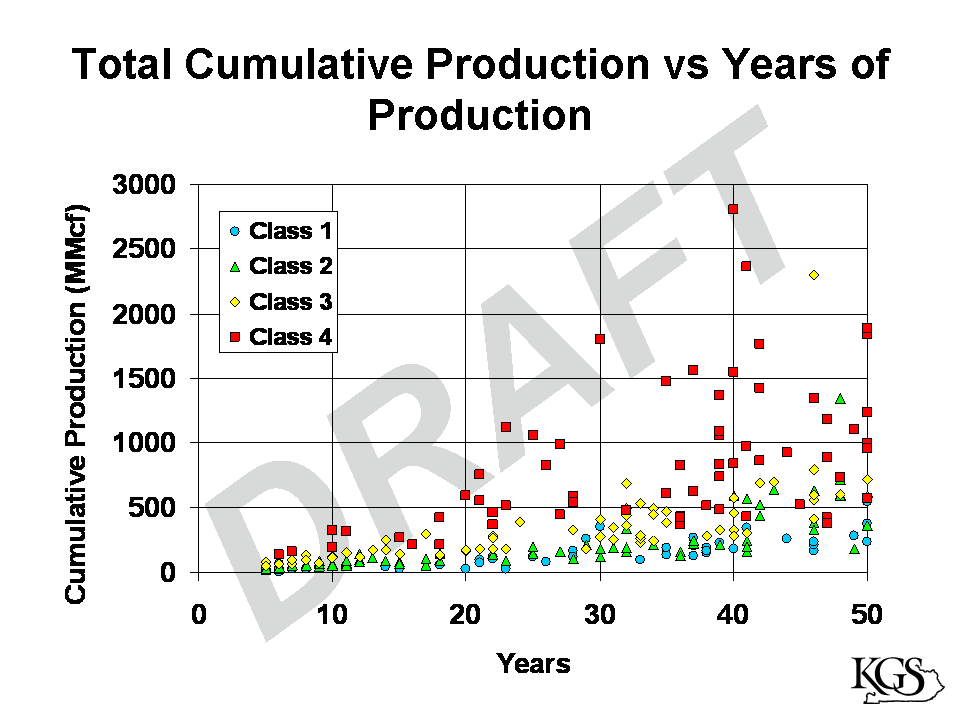 Total cumulative production data can be grouped using percentiles based on the distribution of cumulative production data after 5 years. For example, for those wells that have 20 years of production, the first five years of production show some wells have lower performance (Class I) and some wells exhibit higher performance (Class 4). This chart demonstrates the general persistence of better production over the life of a well based on an assessment of the first 5 years of production data. Total cumulative production data can be grouped using percentiles based on the distribution of cumulative production data after 5 years. For example, for those wells that have 20 years of production, the first five years of production show some wells have lower performance (Class I) and some wells exhibit higher performance (Class 4). This chart demonstrates the general persistence of better production over the life of a well based on an assessment of the first 5 years of production data. |
|
Resources
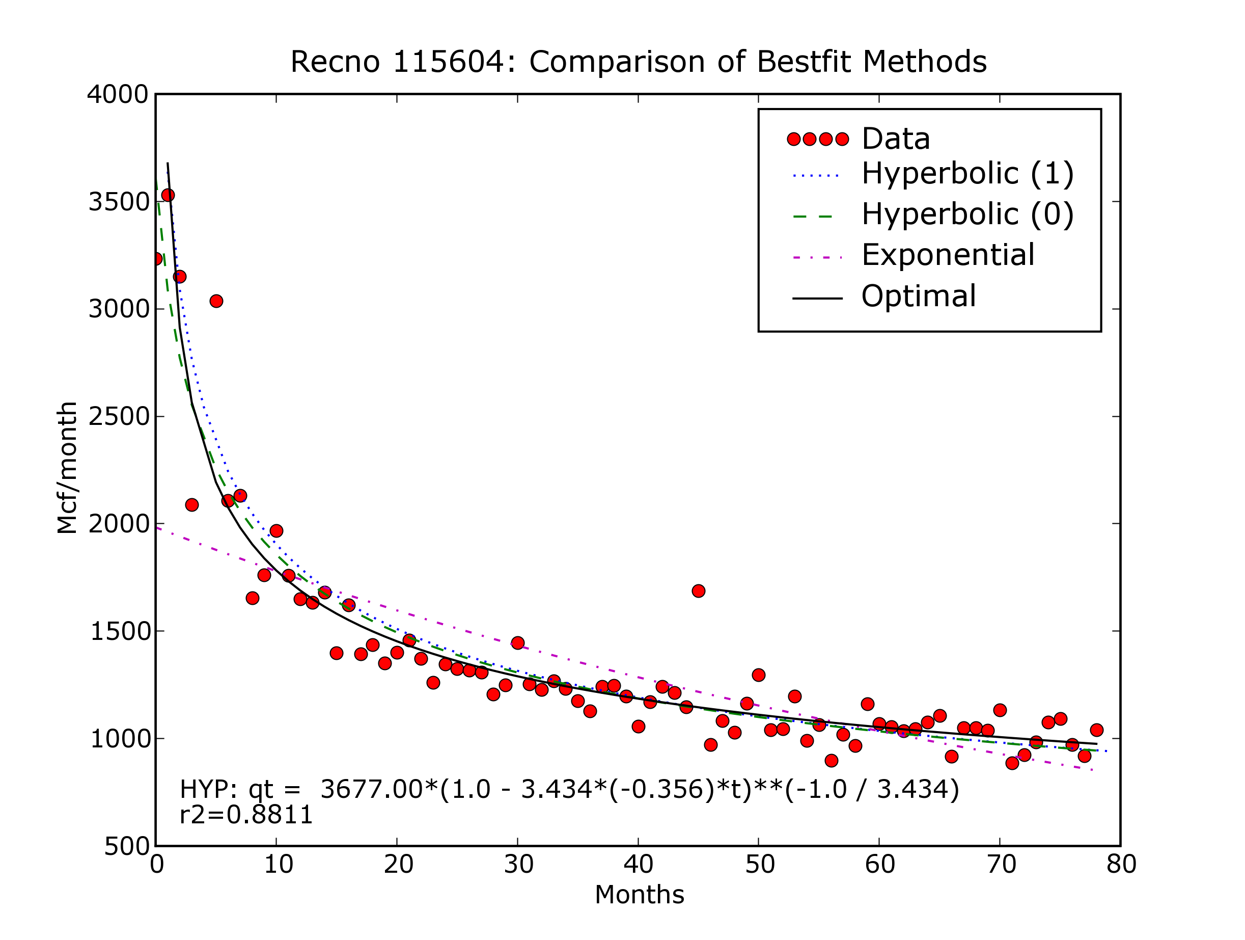
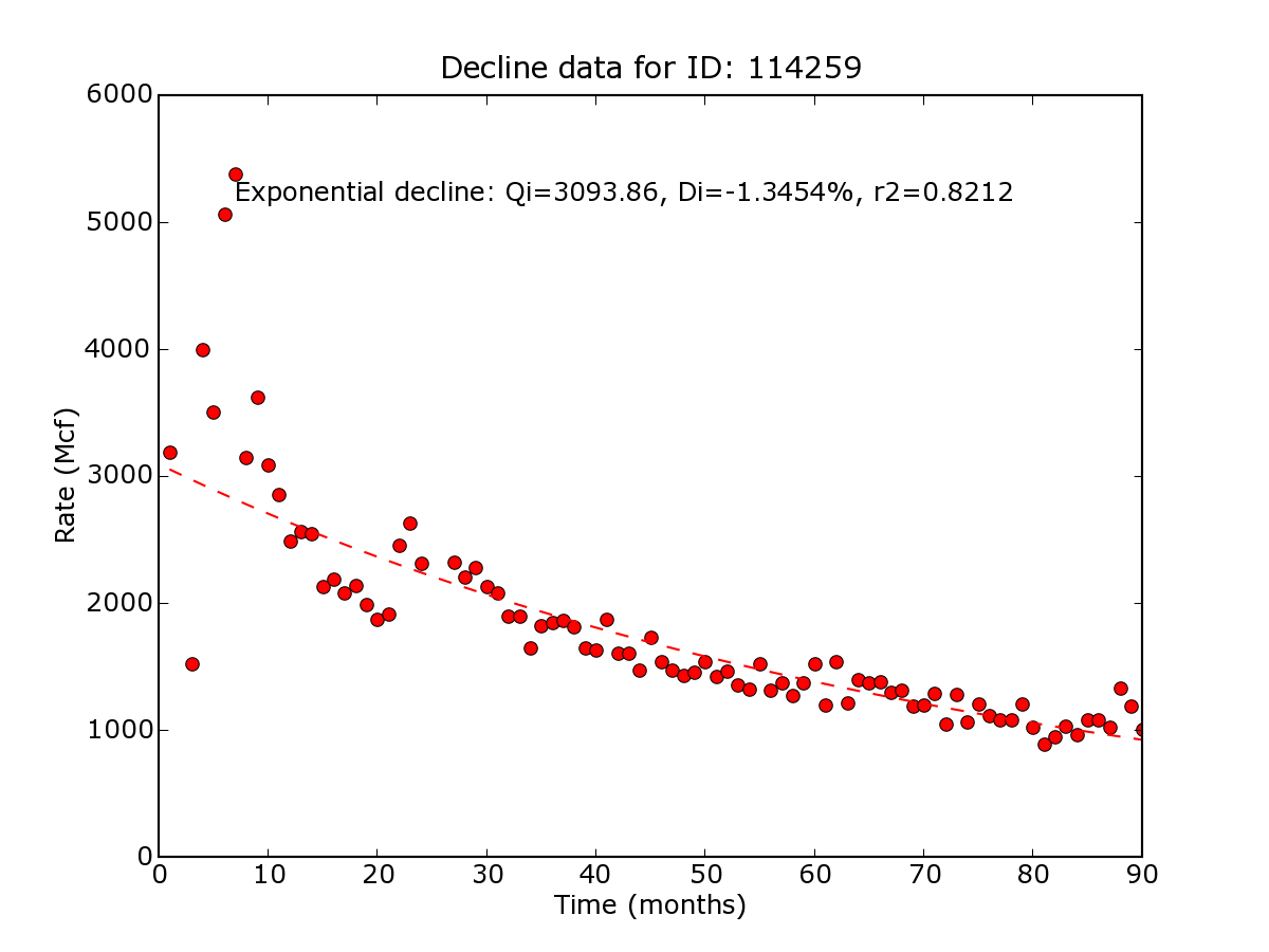
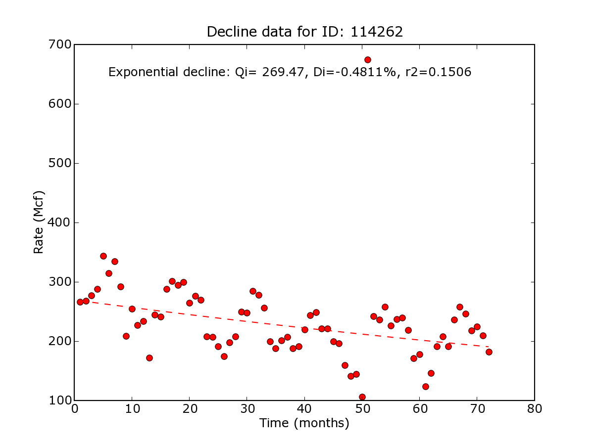
decline_obj.py is the source code for a Python module for interactive or batch processing of rate/time data to determine the best fit hyperbolic or exponential decline parameters. The module can be forced to use a particular model. A method is provided that will iterate over the first few periods of data to see if the best fit can be optimized. Using this capability is suggested if the initial period of production is not the maximum observed production rate. This option can also be used to specify a starting point for the calculations other than the initial period of production. For more information, see the documentation in the file; Python self-documenting features are used. This code was updated 26-Sep-2012 to run under the Enthought Python 2.7.2 distribution.
![]()